Back to the syllabus
ECMJ: First models of climate change
Let's develop a first simple model of climate change. These notes are based on this lecture.
We first need to recall the fundamental concept of differential equation and see how to solve them in Julia.
Differential equations
What is a scientific model? A matematical description of (some aspects of) reality.
What's the language with which such a description can be formulated? It's the language of equations, namely equalities among formulas that impose constraints on what can happen.
What else can we say about how these equations usually look like? Usually, when modeling reality, we are interested in knowing what happens after some time, given some initial conditions. Our equations will likely be functions of a time variable $t$. Moreover, it is typically the case that, rather than being able to describe with an equation how the system look like at a certain time $t$, we only have hypotheses about how the system changes across time: for example, we can rarely predict, a-priori, where a moving mass will be located in space, but we can provide equations that approximate how the position of the mass will change from an instant to the next one.
The equations describing how a function changes are called differential equations.
A simple example of ordinary (one-variable) differential equation is $D_t y = a - bt$. In Julia we can define such differential equation using the ModelingToolkit library:
using ModelingToolkit

@variables t y(t)
@parameters a b
D = Differential(t)

equation = [
	D(y) ~ a - b*t
]

@named system = ODESystem(equation)
Model system with 1 equations
States (1):
  y(t)
Parameters (2):
  a
  b
The @named macro essentially rewrites the last line as
system = ODESystem(equation; name=:example_system)
We can then solve the system with a compatible Julia library of numerical solvers:
using DifferentialEquations

init_condition = [y => 0.0]
time_span = (0.0, 10.0)
parameters = [a => 2.0, b => .5]

problem = ODEProblem(system, init_condition, time_span, parameters)
solution = solve(problem)
retcode: Success
Interpolation: specialized 4th order "free" interpolation, specialized 2nd
order "free" stiffness-aware interpolation
t: 7-element Vector{Float64}:
  0.0
  9.999999999999999e-5
  0.0010999999999999998
  0.011099999999999997
  0.11109999999999996
  1.1110999999999995
 10.0
u: 7-element Vector{Vector{Float64}}:
 [0.0]
 [0.00019999749999999992]
 [0.0021996974999999993]
 [0.022169197499999987]
 [0.21911419749999986]
 [1.9135641974999984]
 [-5.000000000000018]
Let's see the solution:
using Plots
plot(solution, ylim=(-5,5), framestyle=:origin)

The simplest climate model
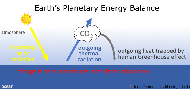
Let's consider arguably the simplest nontrivial climate model:
\[ \begin{align*} & \color{brown}{\text{change in heat content}} \newline &= \color{orange}{\text{incoming solar radiation (energy from the Sun's rays)}} \newline & \phantom{=} - \color{blue}{\text{outgoing thermal radiation (i.e. blackbody cooling to space)}} \newline & \phantom{=} + \color{grey}{\text{human-caused greenhouse effect (trapped outgoing radiation)}}. \end{align*} \]
Each of the above terms should be intended as an average over the entire globe.
Incoming radiation ☀️
Let's address the first term, $\color{orange}{\text{incoming solar radiation}}$.
The amount of energy that Earth receives from the Sun, i.e. Earth's insolation, is
S = 1368 # measured in W/m^2
1368
Part of it is reflected back to space. The measure of such effect is called albedo, and in Earth's case can be estimated to be
α = .3
0.3
Thus, out of the energy S that is received by the Sun, the fraction that it is retained is 1-α.
There's another important correction that we should apply to the above measure of insolation.
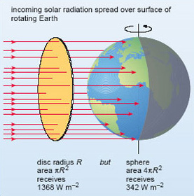
The above number S is estimated for a square meter of surface that lies perpendicularly to the sunrays. However, the Earth's surface is spherical. What's the correction which would apply? A disc of radius $R$ has area $\pi R^2$ while a sphere of the same radius has area $4 \pi R^4$, so there's a factor $\frac 14$ that should multiplay S.
We then have that the incoming solar radiation on the r.h.s. of our starting equation is
in_radiation = S*(1-α)/4;
Earth without outgoing radiation 🔥
Let's start by considering only the $\color{orange}{\text{incoming solar radiation}}$ and ignoring the other terms: $\begin{align*} & \color{brown}{\text{change in heat content}} = \color{orange}{\text{incoming solar radiation}} \end{align*}$
We want to model the Earth's temperature in this simple case:
@variables temp(t)
1-element Vector{Symbolics.Num}:
 temp(t)
The equation above is about the heat content of the planet. 🤔 However, when we enter a swimming pool we don't care about the amount of heat stored in it, we care about the water's temperature, don't we? Recall that the temperature is given by the heat content divided by the heat capacity $C$, in other words
\[ \color{brown}{\text{change in heat content}} = (\color{red}{\text{change in temperature}}) \cdot C. \]
Therefore $\begin{align*} & \color{red}{\text{change in temperature}} = \frac 1C (\color{orange}{\text{incoming solar radiation}} ). \end{align*}$
Hence, in order to estimate how much the incoming radiation will influence the temperature of the Earth, we need to have an estimate the heat capacity of the atmosphere and upper-ocean:
@parameters C = 51. # J/m^2/°C
1-element Vector{Symbolics.Num}:
 C
We thus have the system
@named sys_only_in = ODESystem([ D(temp) ~ in_radiation / C ])
Model sys_only_in with 1 equations
States (1):
  temp(t)
Parameters (1):
  C [defaults to 51.0]
In order to define an ODEProblem, we also need an initial condition. Let's assume that the time 0 of our equation corresponds to the year 1850, before the start of the Second Industrial Revolution; at the time, it is estimated that
temp₀ = 14.0 # °C in 1850
init_condition = [temp => temp₀]
1-element Vector{Pair{Symbolics.Num, Float64}}:
 temp(t) => 14.0
We can now solve system:
prob_only_in = ODEProblem(sys_only_in, init_condition, (0, 170))
sol_only_in = solve(prob_only_in)
retcode: Success
Interpolation: specialized 4th order "free" interpolation, specialized 2nd
order "free" stiffness-aware interpolation
t: 4-element Vector{Float64}:
   0.0
   2.982456140350877
  32.80701754385965
 170.0
u: 4-element Vector{Vector{Float64}}:
 [14.0]
 [27.999999999999993]
 [167.99999999999991]
 [811.9999999999997]
How does the solution look like? Let's plot it:
plot(sol_only_in,
	legend = false,
	xlabel = "Years since 1850",
	ylabel = "°C")
	hline!( [temp₀], ls=:dash)
	annotate!( 80, temp₀,
		text("Preindustrial Temperature = $(temp₀)°C",:bottom))
	title!("Earth's temperature without outgoing radiation")

Earth with outgoing radiation 🥶
Let's move on and consider the $\color{blue}{\text{outgoing thermal radiation}}$, i.e. the black-body radiation which allows Earth to dissipate some of the heat. It is a complicated phenomenon, which we simplify by linearizing it and assuming that, together with the incoming radiation, the overall contribution to $D(\text{temp}(t))$ is equal to $B(\text{temp₀-temp(t)})$ for some $B$:
@parameters B = 1.3 # "climate feedback parameter" in W/m^2/°C
@named sys_in_and_out = ODESystem([
		D(temp) ~ B*(temp₀-temp)/C
	])
Model sys_in_and_out with 1 equations
States (1):
  temp(t)
Parameters (2):
  B [defaults to 1.3]
  C [defaults to 51.0]
This time Earth can cool down. Let's solve the problem assuming that the initial temperature is higher, e.g. 20 °C, and plot the solution:
init_condition = [temp => 20]
prob_in_and_out = ODEProblem(sys_in_and_out, init_condition, (0, 170))
sol_in_and_out = solve(prob_in_and_out)

plot(sol_in_and_out,
	legend = false,
	xlabel = "Years after start",
	ylabel = "°C")
	hline!( [temp₀], ls=:dash)
	annotate!( 80, temp₀,
		text("Initial temperature = $(temp₀)°C",:bottom))
	title!("Earth's temperature with outgoing radiation")

😲 Wow! Unfortunately we are still ignoring one term of our initial equation...
The infamous Greenhouse effect ⛽
The greenhouse effect can be modeled by the equation
\[ \begin{align*} \color{grey}{\text{human-caused greenhouse effect (trapped outgoing radiation)}} \newline = \text{forcing_coefficient} \cdot \ln \left(\frac {\text{CO}_2}{\text{CO}^{(\text{0})}_2}\right), \end{align*} \]
where $\text{CO}^{(\text{0})}_2$ is the initial value of the CO₂ level in the atmosphere.
Empirical data shows that
forcing_coef = 5.0 # W/m^2
CO₂⁽⁰⁾ = 280. # pre-industrial CO₂ concentration, in ppm
280.0
Our prediction of the Earth's temperature will depend on the amount of CO₂ emission; we thus need an hypothesis on the latter. We can extrapolate such hypothesis from past data.

Let's look at data from the Mauna Loa Observatory (more info here):
using CSV, DataFrames

CO2_historical_data_url = "https://scrippsco2.ucsd.edu/assets/data/atmospheric/stations/in_situ_co2/monthly/monthly_in_situ_co2_mlo.csv"
CO2_historical_data = CSV.read(download(CO2_historical_data_url), DataFrame, header=55, skipto=58);

first(CO2_historical_data, 11)
11 rows × 10 columns (omitted printing of 2 columns)
| Yr | Mn | Date | Date | CO2 | seasonally | fit | seasonally | |
|---|---|---|---|---|---|---|---|---|
| Int64 | Int64 | Int64 | Float64 | Float64 | Float64 | Float64 | Float64 | |
| 1 | 1958 | 1 | 21200 | 1958.04 | -99.99 | -99.99 | -99.99 | -99.99 |
| 2 | 1958 | 2 | 21231 | 1958.13 | -99.99 | -99.99 | -99.99 | -99.99 |
| 3 | 1958 | 3 | 21259 | 1958.2 | 315.71 | 314.44 | 316.2 | 314.91 |
| 4 | 1958 | 4 | 21290 | 1958.29 | 317.45 | 315.16 | 317.3 | 314.99 |
| 5 | 1958 | 5 | 21320 | 1958.37 | 317.51 | 314.7 | 317.87 | 315.07 |
| 6 | 1958 | 6 | 21351 | 1958.45 | -99.99 | -99.99 | 317.26 | 315.15 |
| 7 | 1958 | 7 | 21381 | 1958.54 | 315.87 | 315.2 | 315.86 | 315.22 |
| 8 | 1958 | 8 | 21412 | 1958.62 | 314.93 | 316.21 | 313.98 | 315.29 |
| 9 | 1958 | 9 | 21443 | 1958.71 | 313.21 | 316.1 | 312.44 | 315.35 |
| 10 | 1958 | 10 | 21473 | 1958.79 | -99.99 | -99.99 | 312.43 | 315.41 |
| 11 | 1958 | 11 | 21504 | 1958.87 | 313.33 | 315.21 | 313.61 | 315.46 |
We plot the data after removing missing values (here represented by entries $-99.99$):
validrowsmask = CO2_historical_data[:, "     CO2"] .> 0

plot( CO2_historical_data[validrowsmask, "      Date"],
	CO2_historical_data[validrowsmask, "     CO2"],
	label="Mauna Loa CO₂ data (Keeling curve)")
xlabel!("year")
ylabel!("CO₂ (ppm)")

Looking at the data, we guess that the CO₂ in the atmosphere follows the following function (given the current human behavior):
CO₂(t) = CO₂⁽⁰⁾ * ( 1 + ((t-1850)/220)^3 )
CO₂ (generic function with 1 method)
We verify how much our guess overlaps with the data:
years = 1850:2022
plot!( years, CO₂.(years), lw=3,
	label="Cubic Fit", legend=:topleft)
title!("CO₂ observations and fit")

Our guess seems quite good. Let's use it to put the GHE together with the radiation absorbed by the sun, in a complete toy model.
A climate toy model 🌍
Putting everything together we obtain the system
greenhouse_effect(CO₂) = forcing_coef * log(CO₂/CO₂⁽⁰⁾)

@named sys_climate = ODESystem([
		D(temp) ~ (1/C)*( B*(temp₀-temp) + greenhouse_effect(CO₂(t)) )
	])
Model sys_climate with 1 equations
States (1):
  temp(t)
Parameters (2):
  B [defaults to 1.3]
  C [defaults to 51.0]
How fast will the system heat up?
using LaTeXStrings # used in `plot` in `label` property

init_condition = [temp => temp₀]
years = (1850, 2022)
params = [C => 51, B => 1.3]

prob_climate = ODEProblem(sys_climate, init_condition, years, params)
sol_climate = solve(prob_climate)

plot(sol_climate,
	xlabel = "Years after start",
	ylabel = "°C",
	ylim = (10, 20),
	label = L"B=1.3, C=51")

	hline!( [temp₀], ls=:dash, label=nothing)
	annotate!( 1900, temp₀-.8,
		text("Initial temperature = $(temp₀)°C",:bottom))
	title!("Earth's temperature in our toy climate model")

The variables C (heat capacity) and B (feedback parameter) are parameters of ModelingToolkit, meaning that we can try out different values for them, and add some information to the plot:
parameters2 = [C => 20, B => 0.6]

prob_climate2 = ODEProblem(sys_climate, init_condition, years, parameters2)
sol_climate2 = solve(prob_climate2)

plot!(sol_climate2,
	xlabel = "Years after start",
	ylabel = "°C",
	ylim = (10, 20),
	label = L"B=0.6, C=20")

	hline!( [16], ls=:dash, label=nothing)
	annotate!( 1930, 16,
		text("Paris Agreement threshold (2°C warming)", :bottom))

Testing our model 📈
Similarly to what we have done to check our guess for the CO₂ evolution, we can test our overall model against historical data from NASA:
T_url = "https://data.giss.nasa.gov/gistemp/graphs/graph_data/Global_Mean_Estimates_based_on_Land_and_Ocean_Data/graph.txt";
T_df = CSV.read(download(T_url), DataFrame, header=3, skipto=5, delim=" ", ignorerepeated=true);
T_df[1:6, :]
6 rows × 3 columns
| Year | No_Smoothing | Lowess(5) | |
|---|---|---|---|
| Int64 | Float64 | Float64 | |
| 1 | 1880 | -0.17 | -0.1 |
| 2 | 1881 | -0.09 | -0.13 |
| 3 | 1882 | -0.11 | -0.17 |
| 4 | 1883 | -0.18 | -0.2 |
| 5 | 1884 | -0.28 | -0.24 |
| 6 | 1885 | -0.33 | -0.26 |
Let's check our solution sol_climate:
plot(sol_climate[t], sol_climate[temp], lw=2, label="Temperatures predicted by the model", legend=:topleft)
	xlabel!("Year")
	ylabel!("Temperature (°C)")

	plot!( T_df[:,1], T_df[:,2] .+ 14.15, color=:black, label="Observations by NASA", legend=:topleft)
